This chapter describes the use of the general linear model in a wide variety of statistical analyses. If you are unfamiliar with the basic methods of ANOVA and regression in linear models, it may be useful to first review the basic information on these topics in
Elementary Concepts . A detailed discussion of univariate and multivariate ANOVA techniques can also be found in the
ANOVA/MANOVA chapter.
Basic Ideas: The General Linear Model
The following topics summarize the historical, mathematical, and computational foundations for the general linear model. For a basic introduction to ANOVA (MANOVA, ANCOVA) techniques, refer to ANOVA/MANOVA ; for an introduction to multiple regression, see Multiple Regression ; for an introduction to the design an analysis of experiments in applied (industrial) settings, see Experimental Design .
Historical Background
The roots of the general linear model surely go back to the origins of mathematical thought, but it is the emergence of the theory of algebraic invariants in the 1800's that made the general linear model, as we know it today, possible. The theory of algebraic invariants developed from the groundbreaking work of 19th century mathematicians such as Gauss, Boole, Cayley, and Sylvester. The theory seeks to identify those quantities in systems of equations which remain unchanged under linear transformations of the variables in the system. Stated more imaginatively (but in a way in which the originators of the theory would not consider an overstatement), the theory of algebraic invariants searches for the eternal and unchanging amongst the chaos of the transitory and the illusory. That is no small goal for any theory, mathematical or otherwise.
The wonder of it all is the theory of algebraic invariants was successful far beyond the hopes of its originators. Eigenvalues, eigenvectors, determinants, matrix decomposition methods; all derive from the theory of algebraic invariants. The contributions of the theory of algebraic invariants to the development of statistical theory and methods are numerous, but a simple example familiar to even the most casual student of statistics is illustrative. The correlation between two variables is unchanged by linear transformations of either or both variables. We probably take this property of correlation coefficients for granted, but what would data analysis be like if we did not have statistics that are invariant to the scaling of the variables involved? Some thought on this question should convince you that without the theory of algebraic invariants, the development of useful statistical techniques would be nigh impossible.
The development of the linear regression model in the late 19th century, and the development of correlational methods shortly thereafter, are clearly direct outgrowths of the theory of algebraic invariants. Regression and correlational methods, in turn, serve as the basis for the general linear model. Indeed, the general linear model can be seen as an extension of linear multiple regression for a single dependent variable . Understanding the multiple regression model is fundamental to understanding the general linear model, so we will look at the purpose of multiple regression, the computational algorithms used to solve regression problems, and how the regression model is extended in the case of the general linear model. A basic introduction to multiple regression methods and the analytic problems to which they are applied is provided in the Multiple Regression .
The Purpose of Multiple Regression
The general linear model can be seen as an extension of linear multiple regression for a single dependent variable , and understanding the multiple regression model is fundamental to understanding the general linear model. The general purpose of multiple regression (the term was first used by Pearson, 1908) is to quantify the relationship between several independent or predictor variables and a dependent or criterion variable. For a detailed introduction to multiple regression, also refer to the Multiple Regression chapter. For example, a real estate agent might record for each listing the size of the house (in square feet), the number of bedrooms, the average income in the respective neighborhood according to census data, and a subjective rating of appeal of the house. Once this information has been compiled for various houses it would be interesting to see whether and how these measures relate to the price for which a house is sold. For example, one might learn that the number of bedrooms is a better predictor of the price for which a house sells in a particular neighborhood than how "pretty" the house is (subjective rating). One may also detect "outliers," for example, houses that should really sell for more, given their location and characteristics.
Personnel professionals customarily use multiple regression procedures to determine equitable compensation. One can determine a number of factors or dimensions such as "amount of responsibility" ( Resp ) or "number of people to supervise" ( No_Super ) that one believes to contribute to the value of a job. The personnel analyst then usually conducts a salary survey among comparable companies in the market, recording the salaries and respective characteristics (i.e., values on dimensions) for different positions. This information can be used in a multiple regression analysis to build a regression equation of the form:
TOP
Salary = .5*Resp + .8*No_Super
Once this so-called regression equation has been determined, the analyst can now easily construct a graph of the expected (predicted) salaries and the actual salaries of job incumbents in his or her company. Thus, the analyst is able to determine which position is underpaid (below the regression line) or overpaid (above the regression line), or paid equitably.
In the social and natural sciences multiple regression procedures are very widely used in research. In general, multiple regression allows the researcher to ask (and hopefully answer) the general question "what is the best predictor of ...". For example, educational researchers might want to learn what are the best predictors of success in high-school. Psychologists may want to determine which personality variable best predicts social adjustment. Sociologists may want to find out which of the multiple social indicators best predict whether or not a new immigrant group will adapt and be absorbed into society.
Computations for Solving the Multiple Regression Equation
A one dimensional surface in a two dimensional or two-variable space is a line defined by the equation Y = b 0 + b 1 X . According to this equation, the Y variable can be expressed in terms of or as a function of a constant ( b 0 ) and a slope ( b 1 ) times the X variable. The constant is also referred to as the intercept, and the slope as the regression coefficient. For example, GPA may best be predicted as 1+.02*IQ . Thus, knowing that a student has an IQ of 130 would lead us to predict that her GPA would be 3.6 (since, 1+.02*130=3.6). In the multiple regression case, when there are multiple predictor variables, the regression surface usually cannot be visualized in a two dimensional space, but the computations are a straightforward extension of the computations in the single predictor case. For example, if in addition to IQ we had additional predictors of achievement (e.g., Motivation , Self-discipline ) we could construct a linear equation containing all those variables. In general then, multiple regression procedures will estimate a linear equation of the form:
Y = b 0 + b 1 X 1 + b 2 X 2 + ... + b k X k
where k is the number of predictors. Note that in this equation, the regression coefficients (or b 1
b k coefficients) represent the independent contributions of each in dependent variable to the prediction of the dependent variable . Another way to express this fact is to say that, for example, variable X 1 is correlated with the Y variable, after controlling for all other independent variables . This type of correlation is also referred to as a partial correlation (this term was first used by Yule, 1907). Perhaps the following example will clarify this issue. One would probably find a significant negative correlation between hair length and height in the population (i.e., short people have longer hair). At first this may seem odd; however, if we were to add the variable Gender into the multiple regression equation, this correlation would probably disappear. This is because women, on the average, have longer hair than men; they also are shorter on the average than men. Thus, after we remove this gender difference by entering Gender into the equation, the relationship between hair length and height disappears because hair length does not make any unique contribution to the prediction of height, above and beyond what it shares in the prediction with variable Gender. Put another way, after controlling for the variable Gender, the partial correlation between hair length and height is zero.
The regression surface (a line in simple regression, a plane or higher-dimensional surface in multiple regression ) expresses the best prediction of the dependent variable ( Y ), given the independent variables ( X 's). However, nature is rarely (if ever) perfectly predictable, and usually there is substantial variation of the observed points from the fitted regression surface. The deviation of a particular point from the nearest corresponding point on the predicted regression surface (its predicted value) is called the residual value. Since the goal of linear regression procedures is to fit a surface, which is a linear function of the X variables, as closely as possible to the observed Y variable, the residual values for the observed points can be used to devise a criterion for the "best fit." Specifically, in regression problems the surface is computed for which the sum of the squared deviations of the observed points from that surface are minimized. Thus, this general procedure is sometimes also referred to as least squares estimation . (see also the description of weighted least squares estimation).
The actual computations involved in solving regression problems can be expressed compactly and conveniently using matrix notation. Suppose that there are n observed values of Y and n associated observed values for each of k different X variables. Then Y i , X ik , and e i can represent the i th observation of the Y variable, the i th observation of each of the X variables, and the i th unknown residual value, respectively. Collecting these terms into matrices we have
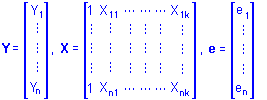
The multiple regression model in matrix notation then can be expressed as
Y = Xb + e
where b is a column vector of 1 (for the intercept) + k unknown regression coefficients. Recall that the goal of multiple regression is to minimize the sum of the squared residuals. Regression coefficients that satisfy this criterion are found by solving the set of normal equations
X'Xb = X'Y
When the X variables are linearly independent (i.e., they are nonredundant, yielding an X'X matrix which is of full rank) there is a unique solution to the normal equations. Premultiplying both sides of the matrix formula for the normal equations by the inverse of X'X gives
(X'X)-1X'Xb = (X'X)-1X'Y
or
b = (X'X)-1X'Y
This last result is very satisfying in view of its simplicity and its generality. With regard to its simplicity, it expresses the solution for the regression equation in terms just 2 matrices (X and Y) and 3 basic matrix operations, (1) matrix transposition, which involves interchanging the elements in the rows and columns of a matrix, (2) matrix multiplication, which involves finding the sum of the products of the elements for each row and column combination of two conformable (i.e., multipliable) matrices, and (3) matrix inversion, which involves finding the matrix equivalent of a numeric reciprocal, that is, the matrix that satisfies
A -1 AA=A
for a matrix A.
It took literally centuries for the ablest mathematicians and statisticians to find a satisfactory method for solving the linear least square regression problem. But their efforts have paid off, for it is hard to imagine a simpler solution.
With regard to the generality of the multiple regression model, its only notable limitations are that (1) it can be used to analyze only a single dependent variable , (2) it cannot provide a solution for the regression coefficients when the X variables are not linearly independent and the inverse of X'X therefore does not exist. These restrictions, however, can be overcome, and in doing so the multiple regression model is transformed into the general linear model.
Extension of Multiple Regression to the General Linear Model
One way in which the general linear model differs from the multiple regression model is in terms of the number of dependent variables that can be analyzed. The Y vector of n observations of a single Y variable can be replaced by a Y matrix of n observations of m different Y variables. Similarly, the b vector of regression coefficients for a single Y variable can be replaced by a b matrix of regression coefficients, with one vector of b coefficients for each of the m dependent variables. These substitutions yield what is sometimes called the multivariate regression model, but it should be emphasized that the matrix formulations of the multiple and multivariate regression models are identical, except for the number of columns in the Y and b matrices. The method for solving for the b coefficients is also identical, that is, m different sets of regression coefficients are separately found for the m different dependent variables in the multivariate regression model.
The general linear model goes a step beyond the multivariate regression model by allowing for linear transformations or linear combinations of multiple dependent variables. This extension gives the general linear model important advantages over the multiple and the so-called multivariate regression models, both of which are inherently univariate (single dependent variable) methods. One advantage is that multivariate tests of significance can be employed when responses on multiple dependent variables are correlated. Separate univariate tests of significance for correlated dependent variables are not independent and may not be appropriate. Multivariate tests of significance of independent linear combinations of multiple dependent variables also can give insight into which dimensions of the response variables are, and are not, related to the predictor variables. Another advantage is the ability to analyze effects of repeated measure factors. Repeated measure designs, or within-subject designs, have traditionally been analyzed using ANOVA techniques. Linear combinations of responses reflecting a repeated measure effect (for example, the difference of responses on a measure under differing conditions) can be constructed and tested for significance using either the univariate or multivariate approach to analyzing repeated measures in the general linear model.
A second important way in which the general linear model differs from the multiple regression model is in its ability to provide a solution for the normal equations when the X variables are not linearly independent and the inverse of X'X does not exist. Redundancy of the X variables may be incidental (e.g., two predictor variables might happen to be perfectly correlated in a small data set), accidental (e.g., two copies of the same variable might unintentionally be used in an analysis) or designed (e.g., indicator variables with exactly opposite values might be used in the analysis, as when both Male and Female predictor variables are used in representing Gender). Finding the regular inverse of a non-full-rank matrix is reminiscent of the problem of finding the reciprocal of 0 in ordinary arithmetic. No such inverse or reciprocal exists because division by 0 is not permitted. This problem is solved in the general linear model by using a generalized inverse of the X'X matrix in solving the normal equations. A generalized inverse is any matrix that satisfies
AA-A = A
for a matrix A.
A generalized inverse is unique and is the same as the regular inverse only if the matrix A is full rank. A generalized inverse for a non-full-rank matrix can be computed by the simple expedient of zeroing the elements in redundant rows and columns of the matrix. Suppose that an X'X matrix with r non-redundant columns is partitioned as
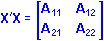
where A11 is an r by r matrix of rank r. Then the regular inverse of A11 exists and a generalized inverse of X'X is
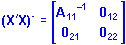
where each 0 (null) matrix is a matrix of 0's (zeroes) and has the same dimensions as the corresponding A matrix.
In practice, however, a particular generalized inverse of X'X for finding a solution to the normal equations is usually computed using the sweep operator (Dempster, 1960). This generalized inverse, called a g2 inverse, has two important properties. One is that zeroing of the elements in redundant rows is unnecessary. Another is that partitioning or reordering of the columns of X'X is unnecessary, so that the matrix can be inverted "in place."
There are infinitely many generalized inverses of a non-full-rank X'X matrix, and thus, infinitely many solutions to the normal equations. This can make it difficult to understand the nature of the relationships of the predictor variables to responses on the dependent variables, because the regression coefficients can change depending on the particular generalized inverse chosen for solving the normal equations. It is not cause for dismay, however, because of the invariance properties of many results obtained using the general linear model.
A simple example may be useful for illustrating one of the most important invariance properties of the use of generalized inverses in the general linear model. If both Male and Female predictor variables with exactly opposite values are used in an analysis to represent Gender, it is essentially arbitrary as to which predictor variable is considered to be redundant (e.g., Male can be considered to be redundant with Female, or vice versa). No matter which predictor variable is considered to be redundant, no matter which corresponding generalized inverse is used in solving the normal equations, and no matter which resulting regression equation is used for computing predicted values on the dependent variables, the predicted values and the corresponding residuals for males and females will be unchanged. In using the general linear model, one must keep in mind that finding a particular arbitrary solution to the normal equations is primarily a means to the end of accounting for responses on the dependent variables, and not necessarily an end in itself.
Summary of Computations
To conclude this discussion of the ways in which the general linear model extends and generalizes regression methods, the general linear model can be expressed as
YM = Xb + e
Here Y, X, b, and e are as described for the multivariate regression model and M is an m x s matrix of coefficients defining s linear transformation of the dependent variables. The normal equations are
X'Xb = X'YM
and a solution for the normal equations is given by
b = (X'X)-X'YM
Here the inverse of X'X is a generalized inverse if X'X contains redundant columns.
Add a provision for analyzing linear combinations of multiple dependent variables, add a method for dealing with redundant predictor variables and recoded categorical predictor variables, and the major limitations of multiple regression are overcome by the general linear model. Top

