Association Rules
Association Rules Introductory Overview
The goal of the techniques described in this section is to detect relationships or associations between specific values of categorical variables in large data sets. This is a common task in many data mining projects as well as in the data mining subcategory text mining . These powerful exploratory techniques have a wide range of applications in many areas of business practice and also research - from the analysis of consumer preferences or human resource management, to the history of language. These techniques enable analysts and researchers to uncover hidden patterns in large data sets, such as "customers who order product A often also order product B or C " or "employees who said positive things about initiative X also frequently complain about issue Y but are happy with issue Z ." The implementation of the so-called a-priori algorithm (see Agrawal and Swami, 1993; Agrawal and Srikant, 1994; Han and Lakshmanan, 2001; see also Witten and Frank, 2000) allows you to process rapidly huge data sets for such associations, based on predefined "threshold" values for detection.
How association rules work.
The usefulness of this technique to address unique data mining problems is best illustrated in a simple example. Suppose you are collecting data at the check-out cash registers at a large book store. Each customer transaction is logged in a database, and consists of the titles of the books purchased by the respective customer, perhaps additional magazine titles and other gift items that were purchased, and so on. Hence, each record in the database will represent one customer (transaction), and may consist of a single book purchased by that customer, or it may consist of many (perhaps hundreds of) different items that were purchased, arranged in an arbitrary order depending on the order in which the different items (books, magazines, and so on) came down the conveyor belt at the cash register. The purpose of the analysis is to find associations between the items that were purchased, i.e., to derive association rules that identify the items and co-occurrences of different items that appear with the greatest (co-)frequencies. For example, you want to learn which books are likely to be purchased by a customer who you know already purchased (or is about to purchase) a particular book. This type of information could then quickly be used to suggest to the customer those additional titles. You may already be "familiar" with the results of these types of analyses, if you are a customer of various on-line (Web-based) retail businesses; many times when making a purchase on-line, the vendor will suggest similar items (to the ones purchased by you) at the time of "check-out", based on some rules such as "customers who buy book title A are also likely to purchase book title B ," and so on.
Unique data analysis requirements.
Crosstabulation tables , and in particular Multiple Response tables can be used to analyze data of this kind. However, in cases when the number of different items (categories) in the data is very large (and not known ahead of time), and when the "factorial degree" of important association rules is not known ahead of time, then these tabulation facilities may be too cumbersome to use, or simply not applicable: Consider once more the simple "bookstore-example" discussed earlier. First, the number of book titles is practically unlimited. In other words, if we would make a table where each book title would represent one dimension, and the purchase of that book (yes/no) would be the classes or categories for each dimension, then the complete crosstabulation table would be huge and sparse (consisting mostly of empty cells). Alternatively, we could construct all possible two-way tables from all items available in the store; this would allow us to detect two-way associations (association rules) between items. However, the number of tables that would have to be constructed would again be huge, most of the two-way tables would be sparse, and worse, if there were any three-way association rules "hiding" in the data, we would miss them completely. The a-priori algorithm implemented in Association Rules will not only automatically detect the relationships ("cross-tabulation tables") that are important (i.e., cross-tabulation tables that are not sparse, not containing mostly zero's), but also determine the factorial degree of the tables that contain the important association rules.
To summarize, Association Rules will allow you to find rules of the kind If X then (likely) Y where X and Y can be single values, items, words, etc., or conjunctions of values, items, words, etc. (e.g., if (Car=Porsche and Gender=Male and Age<20) then (Risk=High and Insurance=High) ). The program can be used to analyze simple categorical variables, dichotomous variables, and/or multiple response variables. The algorithm will determine association rules without requiring the user to specify the number of distinct categories present in the data, or any prior knowledge regarding the maximum factorial degree or complexity of the important associations. In a sense, the algorithm will construct cross-tabulation tables without the need to specify the number of dimensions for the tables, or the number of categories for each dimension. Hence, this technique is particularly well suited for data and text mining of huge databases.
Top
Computational Procedures and Terminology Categorical or class variables.
Categorical variables are single variables that contains codes or text values to denote distinct classes; for example, a variable Gender would have the categories Male and Female .
Multiple response variables. Multiple response variables usually consist of multiple variables (i.e., a list of variables) that can contain, for each observations, codes or text values describing a single "dimension" or transaction. A good example of a multiple response variable would be if a vendor recorded the purchases made by a customer in a single record, where each record could contain one or more items purchased, in arbitrary order. This is a typical format in which customer transaction data would be kept.
Multiple dichotomies. In this data format, each variable would represent one item or category, and the dichotomous data in each variable would indicate whether or not the respective item or category applies to the respective case. For example, suppose a vendor created a data spreadsheet where each column represented one of the products available for purchase. Each transaction (row of the data spreadsheet) would record whether or not the respective customer did or did not purchase that product, i.e., whether or not the respective transaction involved each item.
Association Rules: If Body then Head. The A-priori algorithm attempts to derive from the data association rules of the form: If "Body" then "Head" , where Body and Head stand for simple codes or text values (items), or the conjunction of codes and text values (items; e.g., if (Car=Porsche and Age<20) then (Risk=High and Insurance=High) ; here the logical conjunction before the then would be the Body , and the logical conjunction following the then would be the Head of the association rule).
Initial Pass Through the Data: The Support Value. First the program will scan all variables to determine the unique codes or text values (items) found in the variables selected for the analysis. In this initial pass, the relative frequencies with which the individual codes or text values occur in each transaction will also be computed. The probability that a transaction contains a particular code or text value is called Support ; the Support value is also computed in consecutive passes through the data, as the joint probability (relative frequency of co-occurrence) of pairs, triplets, etc. of codes or text values (items), i.e., separately for the Body and Head of each association rule.
Second Pass Through the Data: The Confidence Value; Correlation Value. After the initial pass through the data, all items with a support value less than some predefined minimum support value will be "remembered" for subsequent passes through the data: Specifically, the conditional probabilities will be computed for all pairs of codes or text values that have support values greater than the minimum support value. This conditional probability - that an observation (transaction) that contains a code or text value X also contains a code or text value Y -- is called the Confidence Value . In general (in later passes through the data) the confidence value denotes the conditional probability of the Head of the association rule, given the Body of the association rule.
In addition, the support value will be computed for each pair of codes or text values, and a Correlation value based on the support values. The correlation value for a pair of codes or text values { X, Y } is computed as the support value for that pair, divided by the square root of the product of the support values for X and Y . After the second pass through the data those pairs of codes or text values that (1) have a confidence value that is greater than some user-defined minimum confidence value, (2) have a support value that is greater than some user-defined minimum support value, and (3) have a correlation value that is greater than some minimum correlation value will be retained.
Subsequent Passes Through The Data: Maximum Item Size in Body, Head. The data in subsequent steps, the data will be further scanned computing support, confidence, and correlation values for pairs of codes or text values (associations between single codes or text values), triplets of codes or text values, and so on. To reiterate, in general, at each association rules will be derived of the general form if " Body " then " Head ", where Body and Head stand for simple codes or text values (items), or the conjunction of codes and text values (items).
Unless the process stops because no further associations can be found that satisfy the minimum support, confidence, and correlation conditions, the process could continue to build very complex association rules (e.g., if X1 and X2 .. and X20 then Y1 and Y2 ... and Y20 ). To avoid excessive complexity, additionally, the user can specify the maximum number of codes or text values (items) in the Body and Head of the association rules; this value is referred to as the maximum item set size in the Body and Head of an association rule.
Tabular Representation of Associations
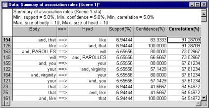
Association rules are generated of the general form if Body then Head , where Body and Head stand for single codes or text values (items) or conjunctions of codes or text values (items; e.g., if (Car=Porsche and Age<20) then (Risk=High and Insurance=High ). The major statistics computed for the association rules are Support (relative frequency of the Body or Head of the rule), Confidence (conditional probability of the Head given the Body of the rule), and Correlation (support for Body and Head , divided by the square root of the product of the support for the Body and the support for the Head ). These statistics can be summarized in a spreadsheet, as shown below.

This results spreadsheet shows an example of how association rules can be applied to text mining tasks. This analysis was performed on the paragraphs (dialog spoken by the characters in the play) in the first scene of Shakespeare's "All's Well That Ends Well," after removing a few very frequent words like is , of , etc. The values for support, confidence, and correlation are expressed in percent.
Graphical Representation of Associations
As a result of applying Association Rules data mining techniques to large datasets rules of the form if "Body" then "Head" will be derived, where Body and Head stand for simple codes or text values (items), or the conjunction of codes and text values (items; e.g., if (Car=Porsche and Age<20) then (Risk=High and Insurance=High) ). These rules can be reviewed in textual format or tables, or in graphical format (see below).

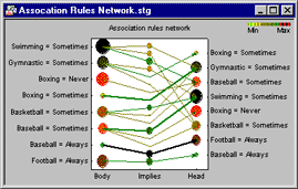
Association Rules Networks, 2D. For example, consider the data that describe a (fictitious) survey of 100 patrons of sports bars and their preferences for watching various sports on television. This would be an example of simple categorical variables, where each variable represents one sport. For each sport, each respondent indicated how frequently s/he watched the respective type of sport on television. The association rules derived from these data could be summarized as follows:
In this graph, the support values for the Body and Head portions of each association rule are indicated by the sizes and colors of each. The thickness of each line indicates the confidence value (conditional probability of Head given Body) for the respective association rule; the sizes and colors of the circles in the center, above the Implies label, indicate the joint support (for the co-occurences) of the respective Body and Head components of the respective association rules. Hence, in this graphical summary, the strongest support value was found for Swimming=Sometimes , which was associated Gymnastic=Sometimes , Baseball = Sometimes , and Basketball=Sometimes . Incidentally. Unlike simple frequency and crosstabulation tables, the absolute frequencies with which individual codes or text values (items) occur in the data are often not reflected in the association rules; instead, only those codes or text values (items) are retained that show sufficient values for support, confidence, and correlation, i.e., that co-occur with other codes or text values (items) with sufficient relative (co-)frequency.

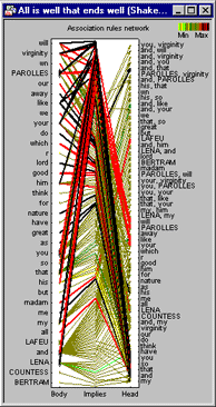
The results that can be summarized in 2D Association Rules networks can be relatively simple, or complex, as illustrated in the network shown to the left.
This is an example of how association rules can be applied to text mining tasks. This analysis was performed on the paragraphs (dialog spoken by the characters in the play) in the first scene of Shakespeare's "All's Well That Ends Well," after removing a few very frequent words like is , of , etc. Of course, the specific words and phrases removed during the data preparation phase of text (or data) mining projects will depend on the purpose of the research.
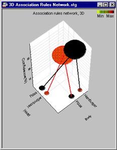
Association Rules Networks, 3D. Association rules can be graphically summarized in 2D Association Networks, as well as 3D Association Networks. Shown below are some (very clear) results from an analysis. Respondents in a survey were asked to list their (up to) 3 favorite fast-foods. The association rules derived from those data are summarized in a 3D Association Network display.

As in the 2D Association Network, the support values for the Body and Head portions of each association rule are indicated by the sizes and colors of each circle in the 2D. The thickness of each line indicates the confidence value (joint probability) for the respective association rule; the sizes and colors of the "floating" circles plotted against the (vertical) z-axis indicate the joint support (for the co-occurences) of the respective Body and Head components of the association rules. The plot position of each circle along the vertical z - axis indicates the respective confidence value. Hence, this particular graphical summary clearly shows two simple rules: Respondents who name Pizza as a preferred fast food also mention Hamburger , and vice versa.
Interpreting and Comparing Results
When comparing the results of applying association rules to those from simple frequency or cross-tabulation tables, you may notice that in some cases very high-frequency codes or text values (items) are not part of any association rule. This can sometimes be perplexing.
To illustrate how this pattern of findings can occur, consider this example: Suppose you analyzed data from a survey of insurance rates for different makes of automobiles in America. Simple tabulation would very likely show that many people drive automobiles manufactured by Ford, GM, and Chrysler; however, none of these makes may be associated with particular patterns in insurance rates, i.e., none of these brands may be involved in high-confidence, high-correlation association rules linking them to particular categories of insurance rates. However, when applying association rules methods, automobile makes which occur in the sample with relatively low frequency (e.g., Porsche) may be found to be associated with high insurance rates (allowing you to infer, for example, a rule that if Car=Porsche then Insurance=High ). If you only reviewed a simple cross-tabulation table (make of car by insurance rate) this high-confidence association rule may well have gone unnoticed.

